How Jev Works Under the Hood: An Illustrated Guide

By Aish Reganti · Published September 22, 2026

A generative LLM writes tokens in sequence; a decision model returns probabilities for supplied choices. The percentages are an example.

Jev is a new model from TypeSafe AI that’s been doing the rounds on social media, with people talking about how fast it is and what they’re building with it. TypeSafe describes it as the first release in a class it calls System One models.

The System One name borrows from the idea of fast, intuitive judgments. For Jev, that means taking some context and questions with defined answers, then returning decisions and probabilities. I’ll use the word decision model to describe this kind of model. ^[1]

For example, we could give Jev a customer’s message and 4 departments, then ask which department should handle it. It would return a department from that list, along with probabilities for the choices. A generative LLM could answer the same question, but it would produce text, even if that text were only a department name or a JSON response.

Jev keeps its output within the choices or values we define. Depending on the question, those outputs take 1 of 3 forms:

Output	What you ask	What comes back
Choice	Which department should handle this?	1 of your supplied departments, probabilities for each option, and confidence.
Score	How urgent is this, using these defined levels?	A numerical rating based on your ordered levels, probabilities for the levels, and confidence.
Noul	Does this customer request a refund?	A number from 0 to 1 representing the probability that the answer is yes.

Those names come from Jev’s question types. For Score, you define what the levels mean. For Noul, 0.8 means an 80% probability of yes.

I was super curious to go a little deeper into the weeds and understand how these models work and how they differ from traditional LLMs. I put together this visual guide to make that easier to follow.

Heads up: since Jev itself isn’t open source, I drew on open-source implementations like Open-Jev and Laya for many of the details below. They help us understand how decision models can be built, though Jev’s exact design isn’t public.

1. How a generative LLM produces text

Before getting into decision models, it helps to refresh how an LLM generates text. We can then follow what changes when the model needs to choose an answer from a supplied set of options.

Let’s use 1 customer message throughout: “My card was charged twice.” First, we ask a generative LLM to draft a reply. It might write, “I can help check the duplicate charge.” We’ll follow how it produces that reply through 3 components, then keep the same numbers when we adapt the model to choose a support department.

Component 1. Tokenization and embeddings

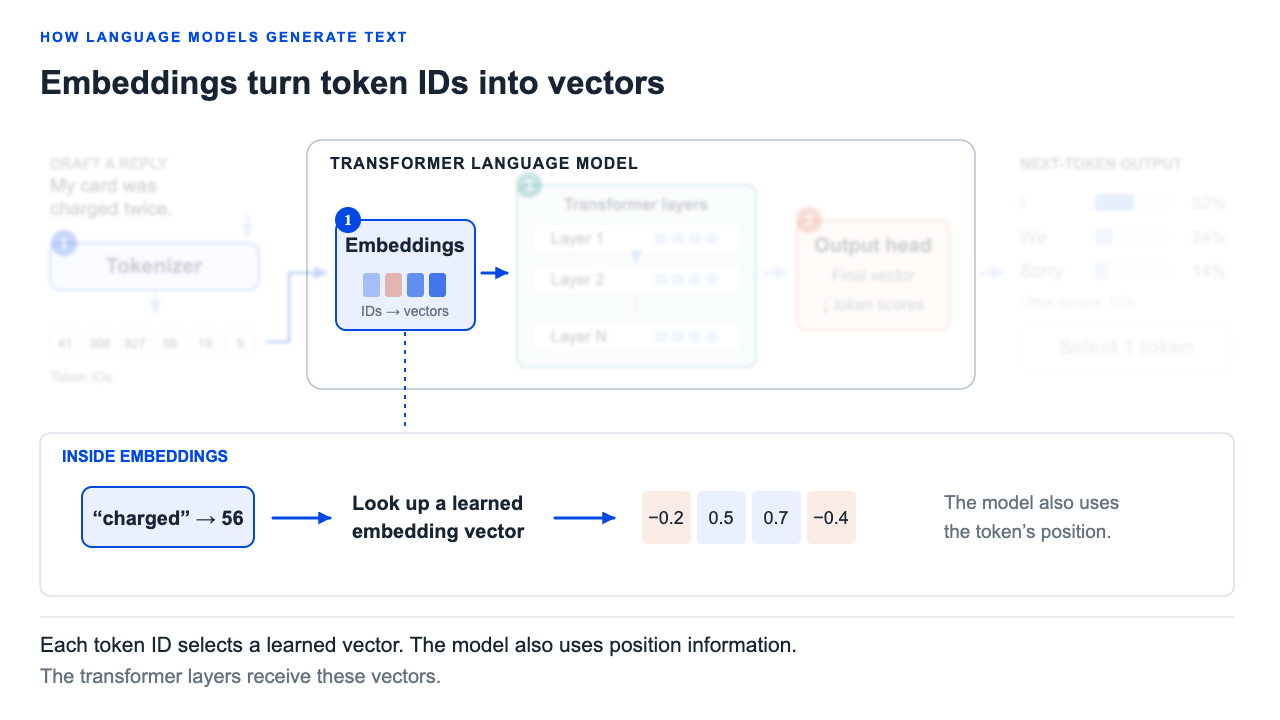
The customer’s message starts as text, which we need to turn into numerical inputs for the model. A tokenizer breaks it into pieces called tokens. For our example, imagine My, card, was, charged, twice, and .. Tokens can also be word fragments or punctuation, and each gets an ID that the model uses to look up an embedding, a list of numbers representing that token.

The tokenizer prepares the input outside the neural network. The embedding layer is inside it. Together, they turn the text into something the model can process.

The customer message becomes token IDs outside the model. Inside the model, embeddings turn those IDs into vectors.

Component 2. The language-processing layers

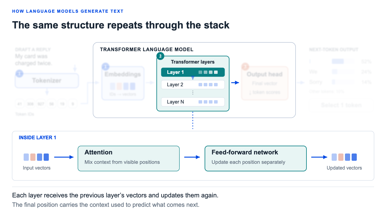
Those embeddings give us an initial representation of each token. As they pass through a stack of layers, often called the backbone, attention lets each position use information from other positions in the available context. A feed-forward network then processes each representation further. The model also accounts for position, because word order matters.

Think of “charged” in “my card was charged twice.” Its surrounding words help establish that we’re talking about a payment. Attention helps the model combine that context as it builds a representation of the message.

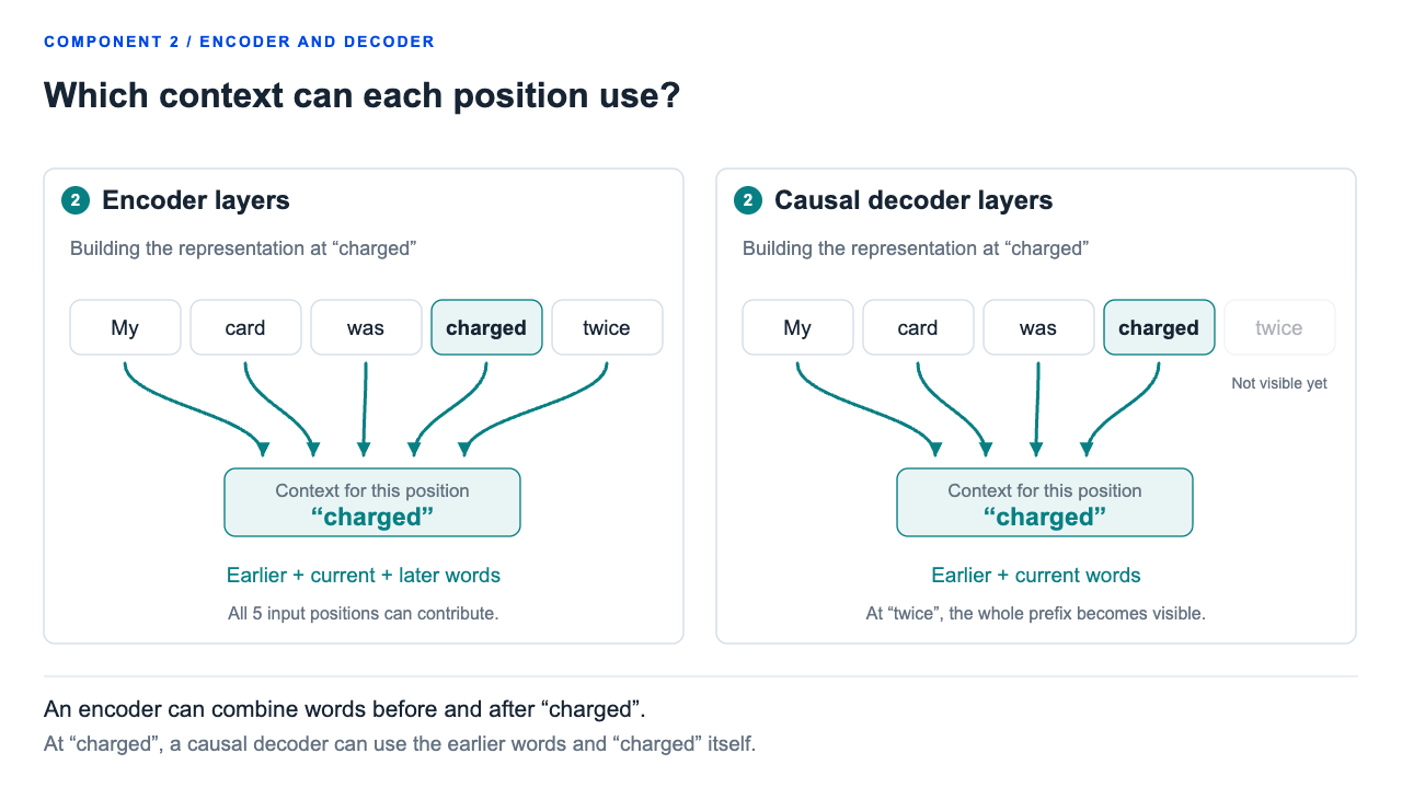
The embeddings pass through transformer layers. Attention combines available context and a feed-forward network updates each representation.

Which surrounding words attention can use depends on how these layers are arranged. 2 arrangements we’ll need to understand are the encoder and the decoder, often described as handling understanding and generation respectively.

Think about listening to someone and then responding. While listening, you’re trying to make sense of what they’re saying. When you respond, you turn what you understand into words, and what you’ve already said shapes what comes next. That’s roughly how the encoder and decoder divide the work in an encoder-decoder model.

An encoder can use context from both directions in the supplied text. A decoder uses the current and preceding positions, which fits continuing a sequence. In an encoder-decoder model, the encoder represents the input and the decoder uses that representation to generate the output. ^[2], ^[3]

But many generative LLMs, including Qwen’s language models, are decoder-only. Their decoder layers also process and interpret the input; they don’t need a separate encoder to do that. So “understanding side” and “generation side” describe their usual roles, rather than 2 halves that every LLM contains. ^[4]

At the word charged, encoder attention can use earlier and later words. Causal decoder attention can use only the current and earlier words.

Component 3. The output head

After those decoder layers have processed the message, we still have numerical representations. To begin writing the reply, the language-model head takes the final position’s representation and scores the possible next tokens across the vocabulary. Those scores become probabilities, and a token is selected.

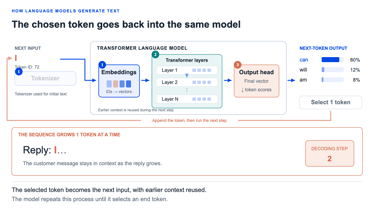
Suppose the first token of the reply is I. It joins the sequence after the prompt, its embedding goes through component 2, and component 3 predicts again. The next token might be can, followed by help, as the model writes “I can help check the duplicate charge.”

Each new token becomes context for the next token. This is the answer-generation loop, also called autoregressive generation. The animation follows the first 3 tokens; the same process continues through the rest of the reply.

During this loop, the model reuses stored information about earlier tokens, so it doesn’t start from scratch each time. It still has to do more computation for every new output token. ^[5]

The vocabulary head selects a next token. That token returns through embeddings and the decoder to predict the following token.

We needed that loop to write a reply. Now suppose the application only needs to route the same message: “My card was charged twice.” We supply 4 departments: billing, fraud, card replacement and general support. The model still needs to interpret the message, but the answer is limited to those 4 options. An LLM can generate a department name; a decision model can score the options directly and return their probabilities.

2. 2 ways to build a decision model

To make that change, we can start with a model that has already learned to process language and adapt it to score decisions. Open-Jev does this with a pretrained decoder, so it gives us a direct comparison with the LLM we just followed. Laya starts with an encoder, which lets us see how a different backbone can serve the same task.

Open-Jev: adapting a decoder

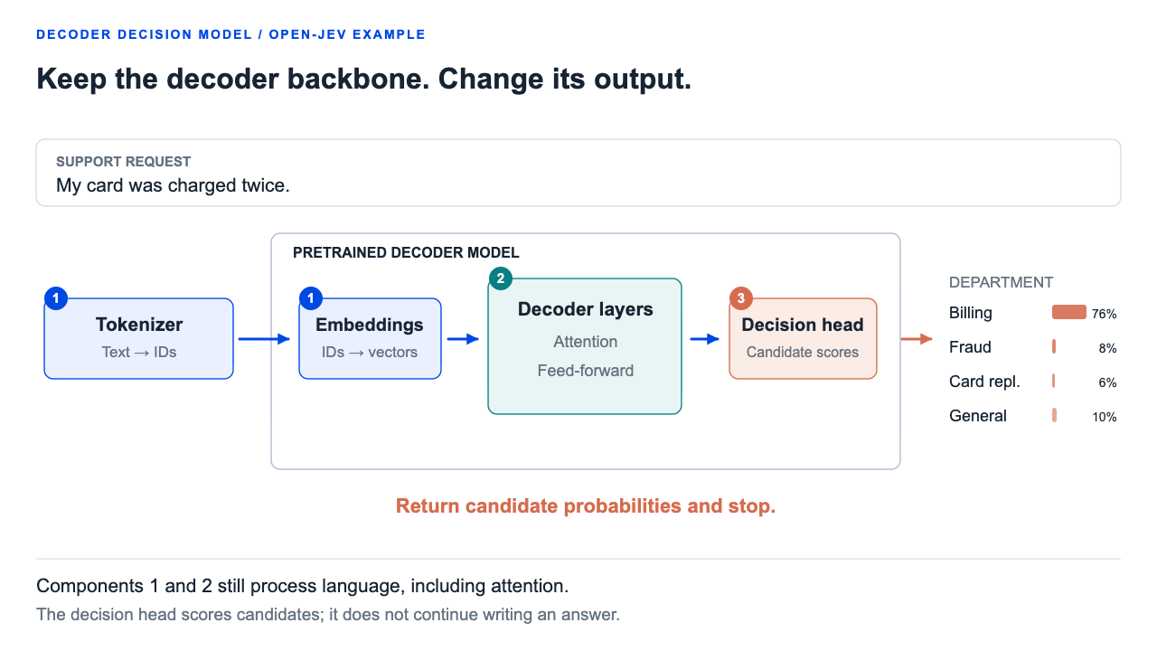
Open-Jev keeps component 1, the pretrained model’s tokenizer and embeddings, and component 2, its language-processing backbone. Together, these components interpret the request and relate it to the possible answers.

Open-Jev replaces component 3, the vocabulary head, with a decision head that scores the supplied candidates. It converts those scores into probabilities without entering the answer-generation loop.

In the Open-Jev example, a decision head replaces the vocabulary head and scores supplied candidates using the decoder representations.

To get a score for each of our 4 departments, Open-Jev constructs a separate input for each proposed answer. Each input contains the customer’s message, the question and 1 candidate answer. The backbone processes each input, and the decision head reads the final position’s representation to produce 1 score. The software combines the 4 scores into probabilities. ^[6], ^[7]

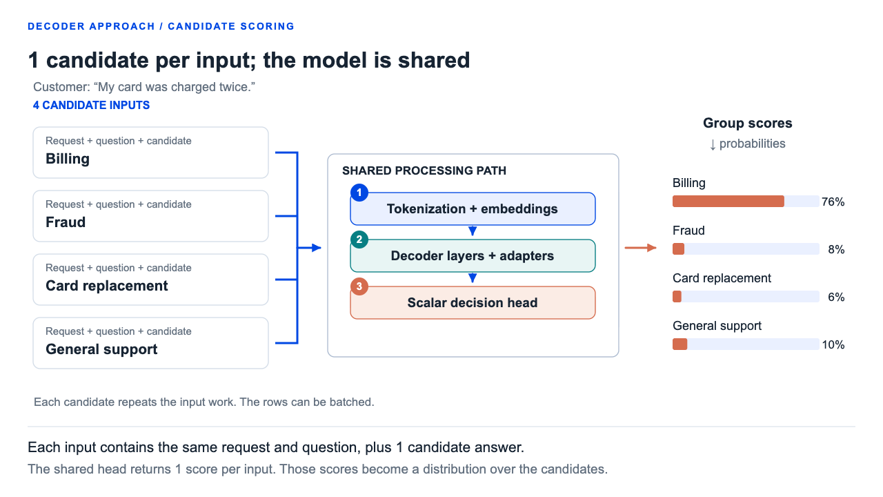
Open-Jev processes the request with each candidate through a shared model. The candidate scores become probabilities over the options.

The new head needs training to produce useful scores. Open-Jev keeps the original backbone weights frozen and trains small additions, called LoRA adapters, alongside the decision head. The adapters adjust how the backbone processes the input, while the head learns to score candidates. ^[8]

Replacing the head is 1 way to get these scores. Eric Zhang’s openjev-sglang makes a lighter adaptation: it keeps component 3 and reads the scores of single-token labels such as A, B, C and D. It avoids continuing the answer, but still computes the vocabulary output. A decision model can therefore retain the vocabulary head, though it still pays the cost of computing those scores.

Laya: adapting an encoder

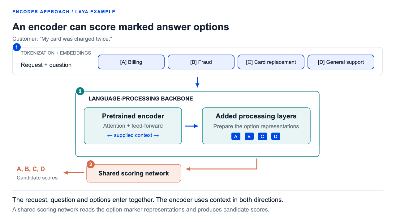
Both of those examples start with a decoder, but scoring supplied answers doesn’t require a model built for continuing text. Laya’s authors start with a pretrained encoder. Their model still uses component 1, tokenization and embeddings, and component 2, language-processing layers with attention. Here, component 2 uses context from both directions in the input, and a decision head fills the role of component 3.

Laya’s English models start from ModernBERT, and their input includes the text, the question and marked answer options.

After the encoder processes them, additional trained layers prepare the representations for scoring. A shared scoring network reads the positions marking the options and produces their scores. So, for our support example, all 4 department descriptions can be represented within 1 question’s input. ^[9]

Attention remains in this approach too, both in the pretrained encoder and in Laya’s added processing layers. Laya avoids generating an answer, while retaining the language-processing layers needed to interpret the text and score the options.

Laya processes the request and marked answer options through an encoder and added layers, then scores the option representations.

Component	Generative decoder LLM	Decoder decision model, as in Open-Jev	Encoder decision model, as in Laya
1. Tokenization and embeddings	Convert text into model inputs	Reuse from pretrained decoder model	Reuse from pretrained encoder model
2. Processing backbone	Decoder layers use current and preceding context	Retain decoder layers, adapted for decisions	Use encoder layers with context in both directions, plus trained processing layers
3. Output head	Score vocabulary tokens	Score supplied candidate inputs	Score marked answer options
Answer-generation loop	Repeat for each output token	Removed	Absent

How this compares with BERT classifiers

If you’ve fine-tuned BERT for classification, a lot of this probably looks familiar. A BERT classifier could already read our support request and predict a department without generating a sentence. In fact, Laya builds on ModernBERT, so there’s a direct connection to the models many ML engineers have worked with.

Remember, though, that a conventional deep-learning classifier often learns a fixed set of labels for a particular task. A model trained to route support tickets has those department labels built into its output head. With these decision interfaces, the question and possible answers arrive with the request. We can ask which department should handle the message, then ask whether it contains a refund request, through the same interface. That makes this a broader way to use classification within an application than training a separate fixed-label head for each task.

There are precedents for that flexibility too. 0-shot natural-language inference models could evaluate candidate descriptions at runtime years before Jev. The BART-MNLI example turns a possible label into a statement and evaluates whether the input supports it. So I see these decision models as building on familiar classification ideas and making them easier to use across different application decisions. The ability to pass in questions and choices helps explain the appeal, but we also need to look at what the returned probabilities mean when software acts on them.

3. Training for calibrated decisions

The decision heads we’ve looked at produce scores that we turn into probabilities. Once software uses those probabilities to decide whether to act, the model’s estimate of certainty becomes part of the application’s behavior. It needs to be evaluated alongside whether the model chooses the right answer.

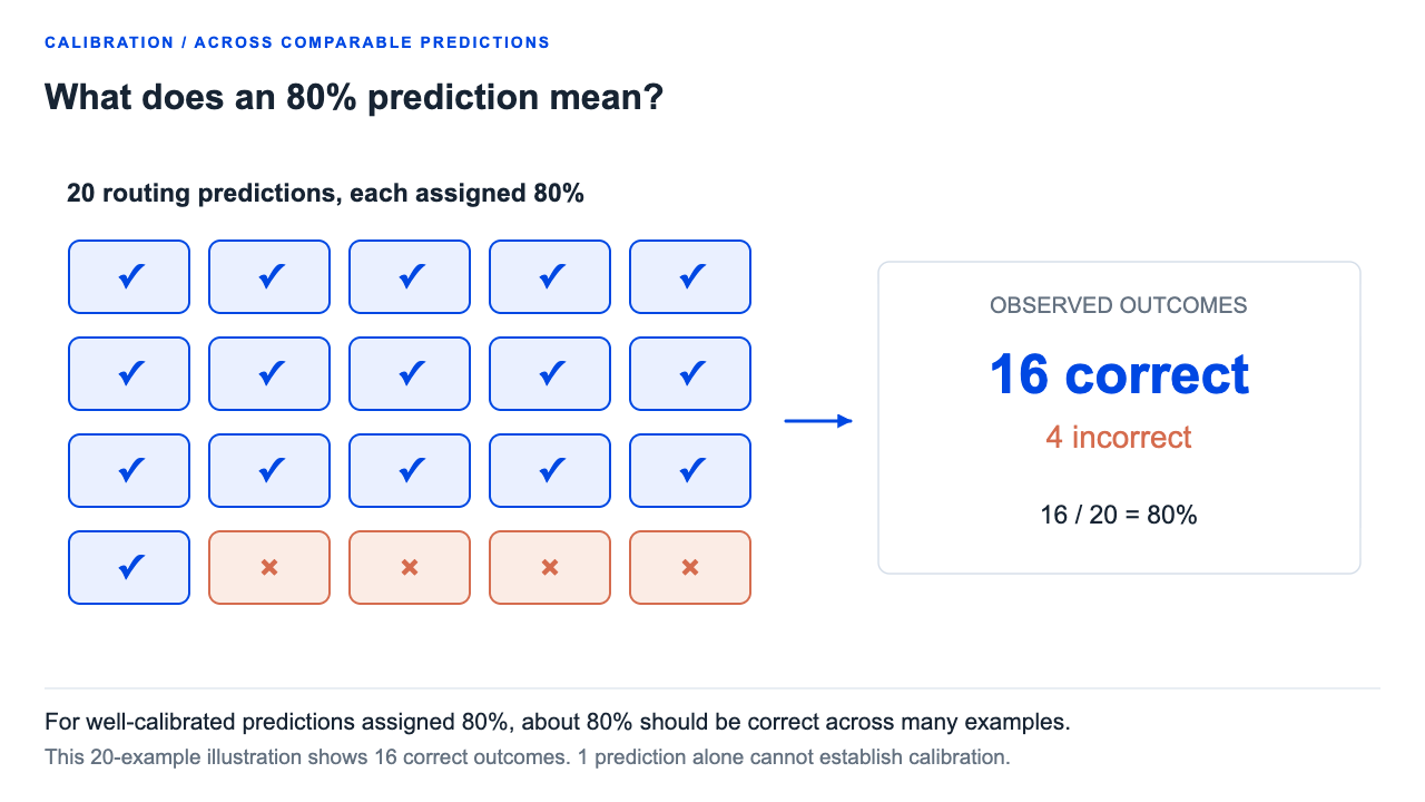
For our routing example, choosing billing is only part of the output. Assigning billing a 60% probability and assigning it 99% communicate very different levels of certainty. Across many comparable support-routing predictions assigned 80%, about 80% should be correct. That is what calibration means; it isn’t a guarantee about 1 individual request.

Across many predictions assigned 80 percent probability, roughly 80 percent should be correct if the probabilities are calibrated.

A generative language model starts by learning to predict tokens, so its next-token probabilities describe what it is likely to write. Restricting the output to answer labels doesn’t establish that those probabilities match how often its decisions are correct. Later training may use human preferences to favor helpful responses, or verifiable rewards to favor answers that pass a check. Those approaches are commonly called RLHF and RLVR.

TypeSafe trains Jev for this probability-estimation task using what it calls Reinforcement Learning for Calibrated Decisions, or RLCD. Its stated training target is decisions accompanied by probabilities that reflect how likely they are to be correct. ^[10]

In reinforcement learning, the model is updated to favor outputs that earn better rewards. For calibrated decisions, the reward needs to account for the probability estimates, including being confidently wrong. TypeSafe has described that objective but hasn’t published the exact reward or update algorithm, so we can’t reconstruct Jev’s training from the name alone.

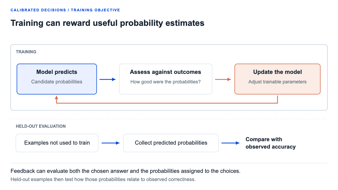
Training for calibrated decisions rewards probabilities that match observed outcomes. This illustrates the objective, not Jev’s unpublished training algorithm.

For an inspectable implementation, we can return to Laya. Its training materials describe probability-scoring rewards and policy-gradient updates, as well as fitting calibration settings using held-out examples. These are Laya’s implementation choices; we don’t know whether Jev uses the same methods. Laya reports overconfidence before calibration and improvement after task-specific training. ^[11]

Older classifiers can also be calibrated, and probability-scoring objectives can be used in supervised learning. To compare them with Jev, we’d need to test both on the same questions, check their probabilities against actual outcomes, and measure their serving costs.

4. Why decision models can be faster and cheaper

Once a model has learned to score the decisions we need, it can return those scores without writing an answer. The architecture changes we followed earlier can save computation in 2 ways:

Removing the answer-generation loop. The model processes the input and scores the choices, then stops. It doesn’t keep running the decoder to write the answer token by token. This is the biggest saving when the alternative is generating a long answer.
Replacing the vocabulary head. A language-model head projects the hidden representation into scores for the entire vocabulary, which can contain 100,000 or more tokens. A decision head only needs to score the candidates. We still convert those scores into probabilities, but over a much smaller set.

For the routing task, we need scores for 4 departments. If we ask an LLM for “billing” plus an explanation or a JSON response, generating that text adds computation. A decision model can return the scores for software to package. The free-form customer reply is a different task: we’d still use a generative model when the application needs to write it.

These changes can reduce the GPU time spent on each request and let the same hardware handle more requests. A smaller pretrained backbone can reduce the computation and memory requirements further.

A decoder-only LLM already has no encoder to remove. Calling a model “decoder-only” therefore doesn’t mean we’ve halved its computation. The savings above come from changing how it produces an answer.

The saving also depends on the workload:

Long documents still require input processing through attention and the other layers.
Large candidate sets can reduce the advantage, especially when an implementation repeats the input for every candidate.
Avoiding a long generated response saves more than avoiding a single-token answer.

Parallel sampling: answering several questions together

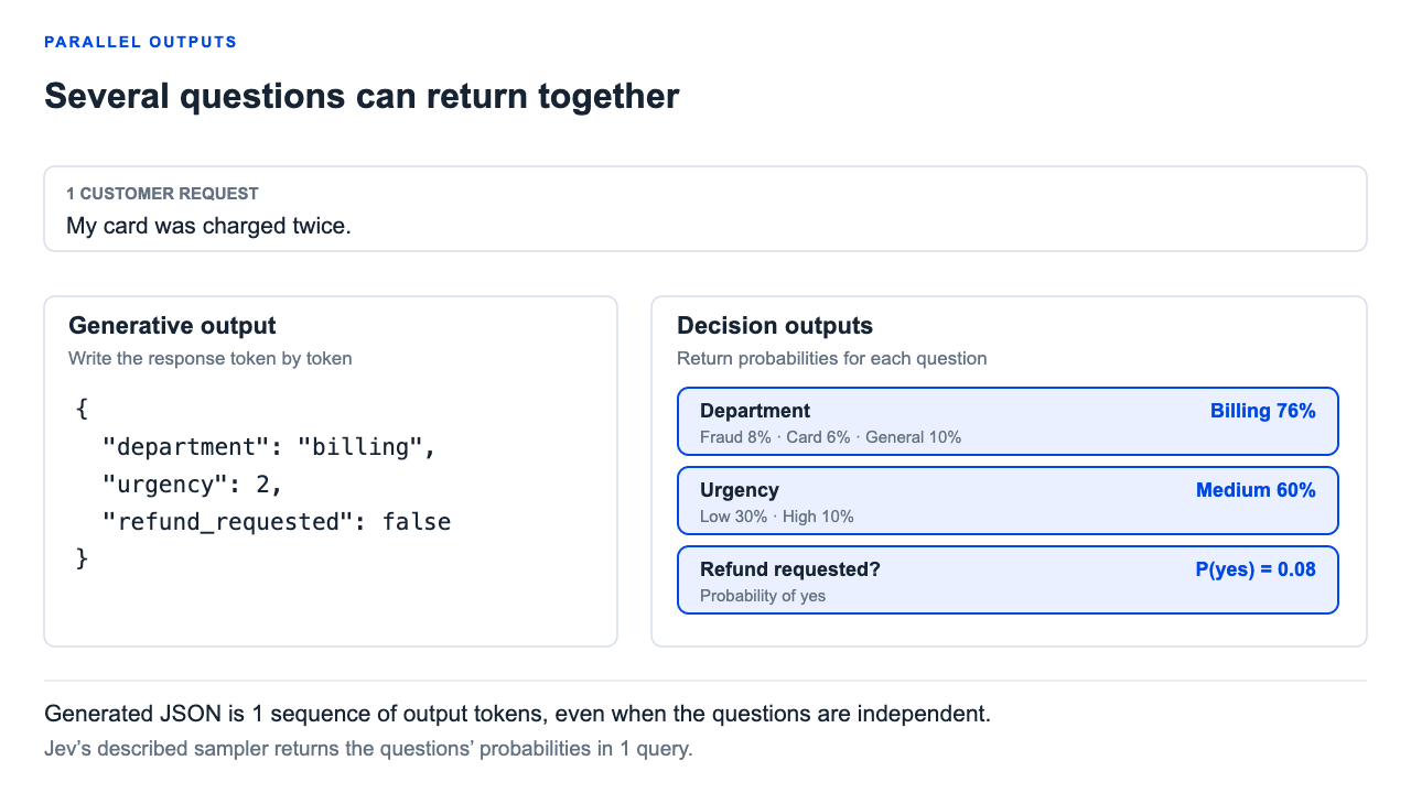
So far, we’ve asked the model to choose a department. The same customer message could also tell us about urgency and whether a refund was requested. A generative LLM returning all 3 in JSON normally writes the result as 1 sequence of tokens. Even though the questions are independent, the output is still generated sequentially.

TypeSafe describes Jev’s parallel sampler as producing the output probabilities for all questions in a single query. The department answer doesn’t have to be written out before the urgency answer can be returned. ^[1]

The open implementations illustrate ways to compute scores together: candidate sequences can be batched in the decoder approach, and question inputs can be batched in the encoder approach. Batching lets the hardware process multiple inputs concurrently. TypeSafe hasn’t published enough detail to equate its sampler with either implementation, or to say that all questions share 1 internal pass.

The model still uses attention to process the inputs. It can then return the decisions together, without writing each answer token by token.

A generative LLM writes JSON token by token. Jev returns probabilities for several questions together in 1 query.

5. Where I think decision models are heading

I do think Jev is a very smart way to package a capability. A lot of the interest makes sense when you realize how many application tasks can be expressed as decisions over a known set of choices. By changing the output space and training a model for those decisions, we can avoid generating an answer token by token and make many of these tasks faster and cheaper.

That starts to look useful in places where calling a generative model for every small decision would be too slow or expensive. Made with Jev is a nice place to see the art of the possible: people are trying these models in routing workflows, browser agents and real-time applications. Looking at that range, I can see why builders are excited about having this kind of capability available through an API.

Over time, though, I do think the wave of standalone decision models might be absorbed by larger model providers. They have a reason to offer cheaper ways to handle the many requests that don’t need a generated response, and I wouldn’t be surprised to see them introduce their own versions in the near future.

As orchestration improves, a provider could offer decision models alongside its generative models and let an application choose what each step needs. Our support workflow could use a decision model to route a request and the other to write a reply, without sending every step through the same expensive model. That’s how I can see this becoming part of a larger model ecosystem, with cheaper options for routine decisions available through the platforms developers already use.